|
|
|
|
|
|
|
|
Paper |
Code |
|
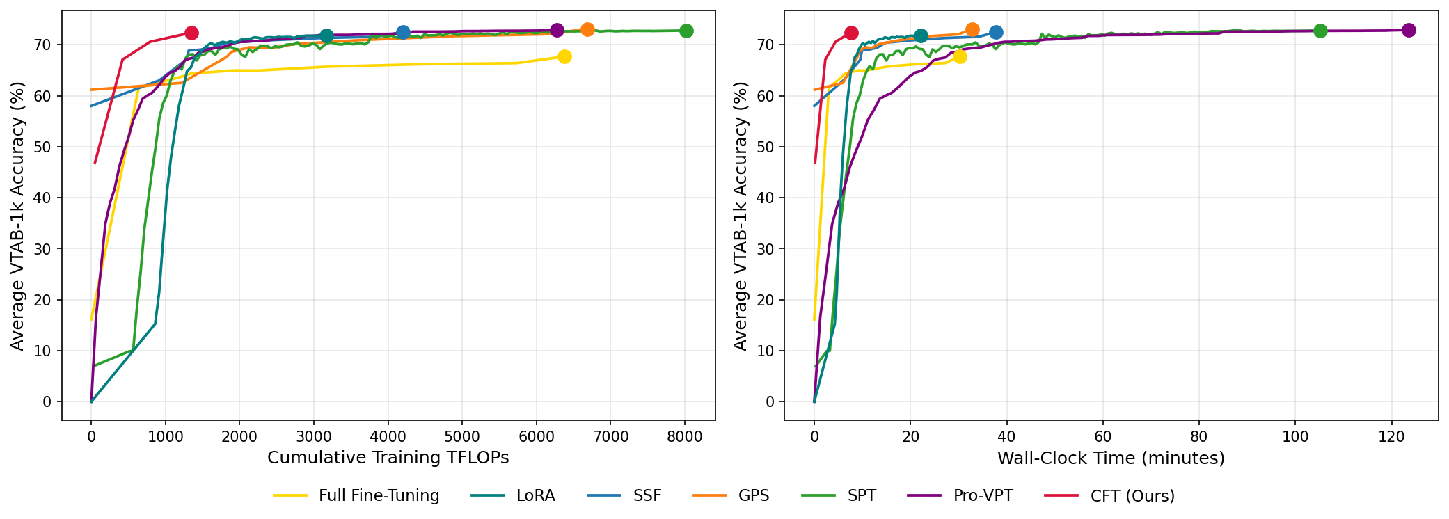
| Parameter-Efficient Fine-Tuning (PEFT) has become the de facto standard for adapting Vision Transformers (ViTs) to downstream tasks. While parameter count has been the dominant efficiency metric in PEFT, it does not imply compute efficiency: parameter-sparse methods can still incur full-model training cost per step, and typically need long schedules to reach peak accuracy. We introduce Circuit Fine-Tuning (CFT), a compute-efficient framework that uses circuit discovery‐conventionally used to explain trained models‐to select modules for fine-tuning before training. Whereas attribution is conventionally formulated against a trained task head, we formulate it against a near-zero-initialized probe head, which isolates the response of the backbone to the target distribution rather than the preferences of a particular classifier. CFT then fine-tunes only the recovered subgraph. CFT needs no learning-rate warmup and reaches peak accuracy in ~20 epochs on average‐versus 44–96 for strong PEFT baselines‐yielding 2.3–6.6× fewer training FLOPs and up to 16× less wall-clock time, while adding zero parameters and no inference operations. Experiments across a standard visual transfer benchmark (VTAB-1k), hierarchical backbones (Swin), domain-shifted medical imaging (CBIS-DDSM), and a vision-language model (Gemma-3 on CUB-200) demonstrate the effectiveness of CFT. |
| CFT consists of two phases. (1) Distribution-aware circuit discovery: using Edge Attribution Patching with Integrated Gradients (EAP-IG) against a near-zero-initialized probe head, we identify the subgraph of attention heads and MLP blocks that the pretrained backbone uses to process the target distribution. The near-zero probe (σ=10−5) suppresses arbitrary class preferences of a random classifier, so importance scores reflect the backbone rather than the head. (2) Sparse circuit adaptation: only the modules in the discovered circuit are fine-tuned; all other backbone modules stay frozen. A fresh classification head is attached and trained with standard AdamW and a cosine schedule‐no learning-rate warmup, no added parameters, and no architectural change. Because CFT only updates values of existing weight tensors, the deployed model is architecturally identical to the original ViT: 1× inference latency, full kernel compatibility (FlashAttention, xFormers, TensorRT, ONNX), and drop-in deployment as a single .pth file. |
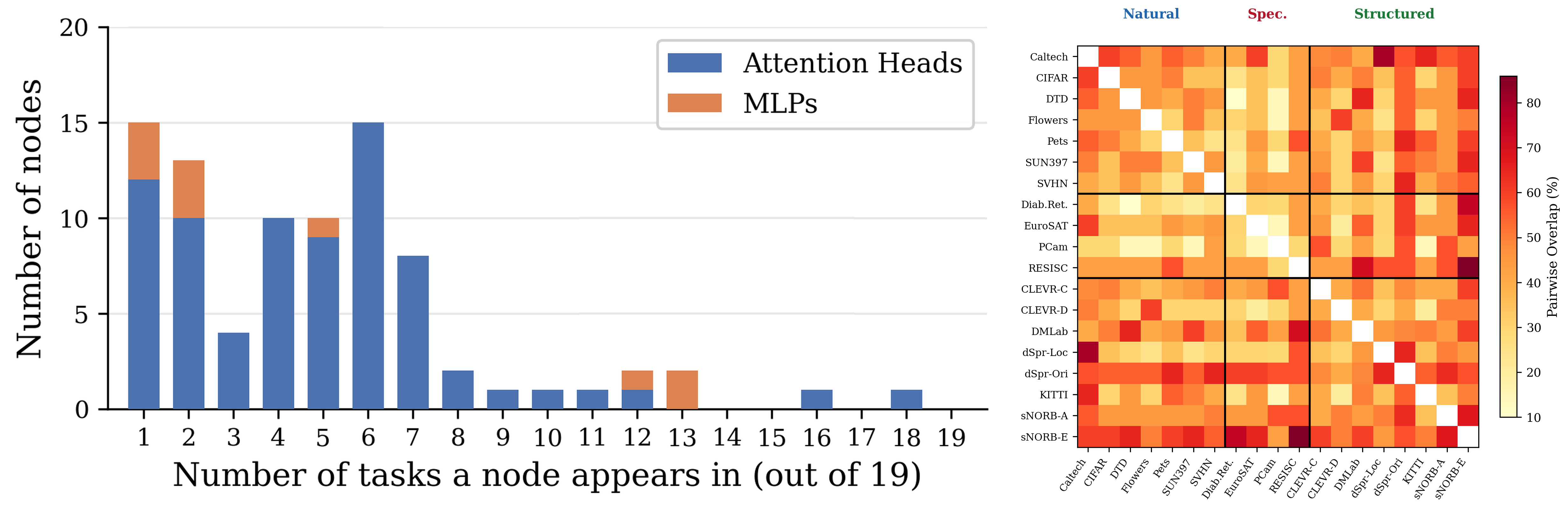
Figure 1. Selected circuits across VTAB-1k tasks (Swin-V2-B). Left: Node selection frequency over the 19 tasks; no node is selected by all tasks, 28 are selected by 1–2, and 6 by ≥12. Right: Pairwise circuit overlap, well above the ~15% expected under random selection at matched budget.
|
Figure 2. CFT reaches high accuracy with far less compute (VTAB-1k, 19-task mean, ViT-B/16). Mean top-1 accuracy vs. cumulative training FLOPs (left) and wall-clock time (right). CFT is the most accurate method across the low-compute range and reaches 72.4 within 1,351 TFLOPs; baselines need 2.3–6.6× more compute to reach their own peaks, which end at most 0.7 points higher.
|
Table 1. Equal epoch budgets with retuned learning rates for each schedule (mean over 6 VTAB-1k tasks, ViT-B/16). Each column is a separate set of runs. CFT is ahead at every budget.
|
Table 2. VTAB-1k training cost (ViT-B/16). TFLOPs and wall-clock time measured up to the best checkpoint of each method. Relative TFLOPs normalized to CFT. % Param. is the fraction of backbone parameters updated, excluding the classification head.
|
Table 3. CBIS-DDSM (mammography, domain-shifted), ViT-B/16 backbone. Fixed 5-epoch budget for all methods.
|
Table 4. VLM adaptation on CUB-200 (Gemma-3-4B-IT), a feasibility study. All fine-tuned methods use the same 5-epoch budget.
|